Thermal Imagery Project Results

Introduction

The following blog post is a continuation of my Project Proposal and Thermal Imagery Collection blog posts.  Throughout this blog post I will display the methods I used to mosaic the imagery. Additionally, I will show the methods I used to display and interpret the results. Another focus of the blog will be on ways to utilize the results for various applications.

Methods

Creating mosaics of the images was the next step after collecting the imagery. As in previous blogs I will be utilizing Pix4D to create the mosaic images. The initial plan was create mosaics without utilizing GCP's and then rerun the image with GCP's. However, plans don't always go the way they are suppose to. I ran all of the flights using Pix4Dmapper Pro version 2.0.104.  Shortly after completing the no GCP mosaics, version 2.1.51 was released which had a Thermal Camera processing option (Fig. 1).

The first results of the mosaics from 2.0.104 were pretty decent but they contained a few errors. I decided to utilize the new version (2.1.51) to run flight 2 again without GCP's to compare the results. The results from 2.1.51 corrected most of the errors contained in the 2.0.104 image (Fig. 2).

(Fig. 2) Flight 2 mosaic with version 2.0.104 (top) with error along the right side with the creek alignment. Flight 2 mosaic with version 2.1.51 (bottom) and the error along the creek has been remedied.

 I ran the remaining images again without GCP's with the considerable improvement in the flight 2 results. All went well until I attempted to run flight 5 and got an error (Fig. 3)

(Fig. 3) Error in the Log Output while running flight 5.

My professor and I various attempts to rerun the images making alterations to various settings to no avail. We sent a message to Pix4D technical support, and receive a reply stating the Thermal Camera Processing option was designed to run nor did they support the resolution (336x225) of our camera. They did not have any explanation as to why the first 4 flights ran other than luck. So, the results from flights 1 through 4 produced with version 2.1.51 will be the basis of my assessment.

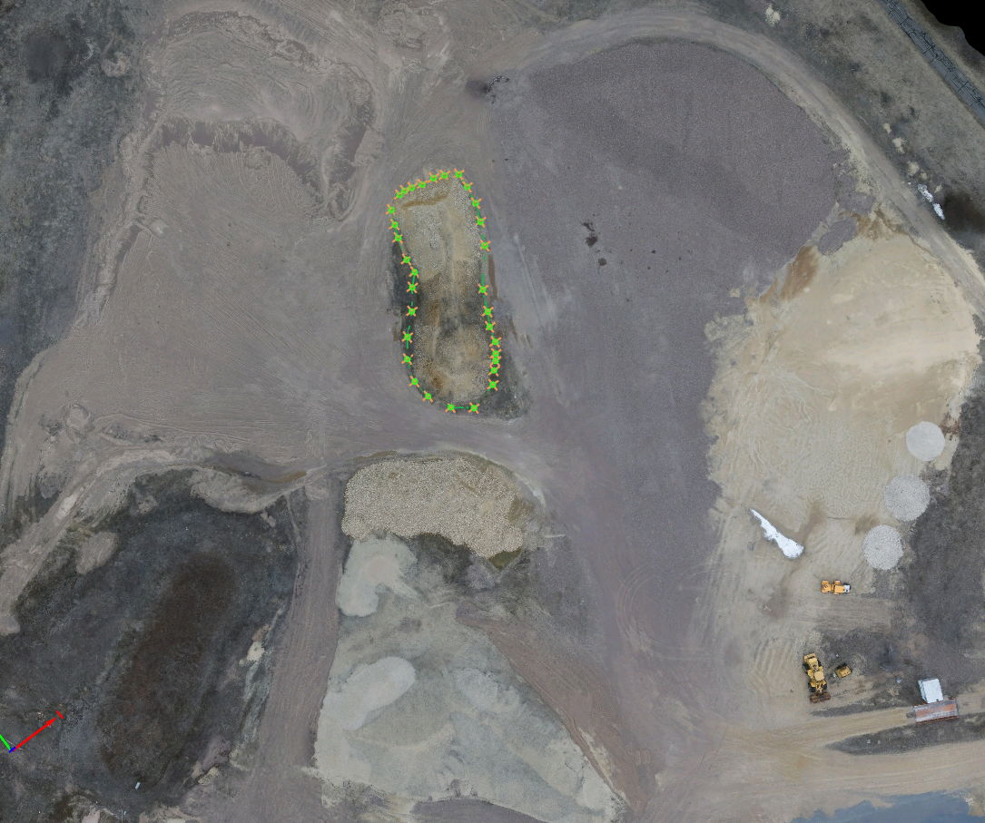
To display the diurnal change of the surface temperatures I opened the .tiff image in ArcMap. The original symbology display did not accurately display the change between the imagery.  I changed the Stretch type to Minimum-Maximum and matched the display values through the Layer Properties menu (Fig. 4).

(Fig. 4) Symbology stretch type set to Minimum-Maximum.

Results

(Fig. 5) Display of the mosaic images from the flights.

(Fig. 6) Chart displaying the collected surface temperature values collected.

(Fig. 7) Chart displaying the soil temperature values collected.

Discussion

The results display the diurnal change of the temperatures very well.  Focusing on the roof of the house you can see the transition from the sun being in the eastern sky in the morning to the western sky in the afternoon (Fig.8)

(Fig. 8) Display of the roof temperature change between flight 2 which was collected at 9:00 am and flight 4 which was collected 3:00 pm.

The original color ramp and stretch effect I selected displayed the diurnal change the best. I determine with the stretch set to Percent Clip and a more variable color ramp showed variations in the surface temperatures better for certain surfaces such as the blacktop road and the vegetated areas while experimenting with colors variations (Fig. 9). Notice the roof of the house does not display the same distinct variations as the previous color ramp for flight 4.

(Fig. 9) Display of the imagery with stretch set to Percent Clip and altered color scheme for flight 4.

When analyzing the image I noticed you could see the cracks on the road surface (Fig. 10). There are numerous application such as, surveying the quality of roads or estimating the time it would take to repair the road surface.

(Fig. 10) Clipped image of the road surface displaying the cracks in the road ways from flight 4.

Examining Fig. 9 further you can see variations in the vegetated surfaces and the farm field on the west side of the road. You can notice the tilled farm field is displaying a warmer temperature compared to the vegetated areas on the east side of the road. These type of results could be utilized for land management and educational purposes when displaying the effects of ground cover compared to bare soil.

While these results are very exciting and are very useful. The next step is to determine a method/algorithm to determine the true surface temperature values from the UAS imagery. Additionally, we will be sending our thermal camera in for upgrades to the resolution which will all us to process the imagery in Pix4D and have higher quality results.

I will be working with Dr. Cyril Wilson and Dr. Joseph Hupy this summer to develop the algorithm to extract the true surface temperature values for the imagery. To stay up to date on our progress make sure to visit my UAS Field Journal which will contain progress of my internship along with other various UAS happenings throughout the summer including thermal processing updates.

Volumetrics with Pix4D and ArcMap

Introduction

Dr. Hupy has been displaying to us that the applications for UAS are expanding daily.  The utilization of UAS to calculate the volume of stock piles in aggregate mining operations is one of the new application Dr. Hupy has been exploring. Calculating the volume of piles with UAS is more effective in both time and cost. Reducing the cost of could result in higher frequency of stock pile assessments and/or an overall cost savings for the business.  Throughout this lab I will be calculating the volume for 3 different stockpiles using 3 different methods.  I will then compare the results between the 3 different methods.

Methods

Per the instruction of my lab assignment i will be calculating the volume of 3 different aggregate piles at the Litchfield mine site using 3 various methods.  The first method will utilize the volume tool in Pix4D which I have used previously. I will utilize ArcMap to calculate a raster volume first, and then calculate the volume of a Triangulated Irregular Network (TIN). I will use the mission from the Litchfield Mine which was collected with 24 megapixels and flown at a 200 foot elevation from our class held on 3/13/2016 to select my piles from and calculate the volume (Fig. 1).

(Fig. 1) Display of the three piles I will be analyzing from the Litchfield flight.

Pix4D

Pix4D has the simplest process to calculate the volume of the piles. I will be utilizing the same method to calculate the volume in Pix4D as I did in my previous blog post. I created 3 separate volume perimeters in Pix4D (Fig.2).  Once the adjusted volume was displayed I recorded the value in an Excel spreadsheet.

(Fig. 2) Volume perimeters created in Pix4D with display window.

Raster Volume

I first had to digitize polygons of the same piles used in the volume calculation Pix4D. I completed the task using the Editor function after opening the mosaic image produced by Pix4D in ArcMap (Fig 3). I then opened the Digital Surface Model (DSM) created by Pix4D in the same data frame of ArcMap. I then utilized the polygon feature to Extract by Mask each area of the piles separately from the DSM (Fig. 4). Using the identify tool I selected pixels at the base of the pile to determine the base height for the pile which I recorded on paper for the next step. The next step was to calculate the surface volume of the pile using the Surface Volume tool in ArcMap. With the Surface Volume window open I set the Input Surface to the clipped DSM image for the first pile, Output Text File was set to my folder, Reference Plane set to ABOVE (as the plane height will be set to the bottom of the pile), Plane Height is set to the dimension I recorded in the previous step (Fig. 5). After selecting OK a text file is created and when opened displays the volume for the pile. The workflow is the same for all 3 piles (Fig. 6).

(Fig. 3) Digitized polygons of the analyzed piles in ArcMap.

(Fig. 4) Extracted polygons of the piles from the DSM image.

(Fig. 5) Surface Volume window with parameters set.

(Fig. 6) Workflow for calculating the volume of a raster segment (Bomber 2015).

TIN Volume

First I converted the clipped raster pile sections to a TIN utilizing the Raster to TIN tool in ArcMap. When the TIN is created no information is transfer to the feature. I needed to attach information related to the elevation to the TIN file. I used the Add Surface Information tool to add the z_mean and z_min field to the TIN files of each of the piles. After researching and talking with classmates I determined the z_min field was the one I need to utilize when calculating the volume of the TIN.
I used the Polygon Volume tool to calculate the volume of the TIN's. The parameters of the tool were set to the following: Input Surface was set to the created TIN for pile 1, Input Feature Class was the DSM clipped segment of pile 1, Height Field was set to the z_min from the previous step, Reference Plane was set to ABOVE (again as the reference height was based at the bottom of the pile (z_min)), Volume Field was left as the default of Volume (Fig 7). After running the tool the TIN calculations are automatically added to the ArcMap window (Fig. 8). The workflow was the same for all three of the piles (Fig. 9).

(Fig. 7) Polygon Volume window with parameters set.

(Fig. 8) TIN calculations displayed in ArcMap.

(Fig. 9) Workflow for TIN volume calculation (Bomber 2015).

Results

Looking at the table I created in Excel you can see variation between the methods used for calculation.

Discussion

The first thing to discuss is the variation between the Pix4D results and the Raster/TIN volume done in ArcMap.  The polygons used between the two were not exactly the same.  I had to draw them separately in both programs thus leading to variations between the results. However, this does not explain the variation in the results between the Raster and the TIN volume as they both utilized the same polygons (sort of) for the calculation. I feel the variation is related to the construction of the TIN polygon.  The TIN is created by average elevation by which triangles are created. I believe the average elevation calculation is to blame for the variation as it is an average and is not the true elevation for the entire pile.  Additionally, the base level set for the ArcMap calculations was an average of the pile base height and did not take into account the slope of the ground (One side of the base was at a different elevation than other sides). More experimentation is required to determine the best method in calculating the volume of stock piles at aggregate mines.

Thermal Imagery Collection

Introduction

The purpose of the weeks assignment was to collect the data for my final project which is based off my project proposal. We flew flights at three hours intervals collecting thermal imagery with the UAS platform. The first three flights and the last flight of the day were conducted with Mr. Mike Bomber, Dr. Joseph Hupy, and myself. We were joined for the 3:00 pm flight by the rest of the UAS class who were collected additional data for their own purposes.   Additionally, I collected in situ surfaces and soil temperature values immediately following the flights. The following blog post will display the methods we utilized to collect the data.



Methods

The collection of data started at 6:00 am on 4/18/2016 (Though the first flight did not get launched till shortly before 6:30). The same process was completed every three hours for a total of 5 flights and temperature values collected. I utilized the Matrix platform fixed with the thermal sensor we have used in previous lab exercises. I created a flight mission which covered my study area thoroughly while maintaining a short enough flight time to complete the mission in one flight. Dr. Hupy laid out 6 portable GCP markers and collected their locations with the dual frequency GPS in hopes of being able to see them in the imagery (Fig. 1).

Collecting surface and soil temperature values was the second step of the process. I determined my sample location prior to the first flight (Fig. 1). My sample sights were based on varying surfaces.  The surfaces included:

• Blacktop
• Mowed Lawn
• Prairie Grass
• Garden area with straw covering the soil
• Garden area with woodchips & straw covering the soil
• Wooden deck surface
• Roof with asphalt shingles
• Conventionally tilled farm field
• Wood chip pile
• Raised garden bed soil not covered

(Fig. 1) Display of the GCP marker locations and the temperature sampling locations in the study area.

I collected surface temperatures immediately following the completion of the flight utilizing an infrared thermometer (Fig. 2). Simultaneously, I collected soil temperatures from the same location utilizing probe thermometer. I will be utilizing the surface temperatures to calibrate the image values to display the temperature change of the surfaces throughout the day. I hope the soil temperature values will display the correlation to soil coverage and the reduction of temperature values.

(Fig. 2) Thermal infrared thermometer utilized to collect surface temperature values

Results

The final results have not been produced yet. I have completed the first step of creating a mosaic image in Pix4D software (Fig 3).  The remainder of the research will be conducted in the up coming weeks.

(Fig. 3) Display of the mosaic image from the 12:00 PM flight.

Litchfield Mine GCP Placement 4/11/2016

Introduction

The purpose of the class on April 11th was to place permanent GCP's at the Litchfield Mine site. Our professor Dr. Joe Hupy recently was awarded the Regent Scholar award from the University Wisconsin System Board of Regents'.  The award is to facilitate exploration in assessing inventory of aggregate mines. Dr. Hupy created a partnership with The Kraemer Company to access a aggregate mine site near the city of Eau Claire.  The access will allow Dr. Hupy and the researchers to continually fly UAS missions to assess the stock piles of aggregate materials at the site. GCP's are one of the components required for the accuracy needed to complete volumetrics of the aggregate piles. The goal was to place the GCPs all around the mine site where they will remain visible for all future flights.

Methods

During last weeks class time we built our own GCP markers.  Dr. Hupy purchased 4 ft by 8 ft sheets of 1/4 inch thick black plastic. We cut the sheets down to 2 ft by 2 ft squares.  We then cut a triangle out of a piece of plywood which was the same size at the plastic.  The triangle was used as a stencil to create the GCP point in the middle of the sheet (Fig. 1).

(Fig. 1) Plywood with triangle cut out laid over top of the black plastic 2x2 plastic sheet.

We then used florescent green spray paint to color in the triangle.  After letting the first side dry we flipped the plywood sheet the opposite direction to create and "hour glass" shape on the sheet (Fig. 2). Additionally, we added letters to each marker for data tracking purposes. The last step was to drill holes in the corners for anchoring purposes.

(Fig. 3) Completed GCP marker with painted triangle and letter.

Now we had to place the GCP markers.  We met at the Litchfield mine in the afternoon of 4/11/2016. We were met by a representative from Kraemer to help us select appropriate locations to place the GCP markers which would not impede their production operation.

After placing and anchoring the marker we utilized a dual frequency GPS to collect the location (Fig. 4). We completed the same task for all of the place GCP markers.

(Fig. 4) Collection of the location of the GCP marker using the dual frequency GPS.

Results

(Fig. 4) Display of placed GCP Markers at the Litchfield mine site.

Project Proposal

Introduction

The research for the project will focus on the use and functionality of the thermal sensor. The thermal sensor does not produce true temperature readings for ground surfaces. I hope through the collection of in situ temperature data from various surfaces on the ground immediately after the flight will allow calibration of the temperatures from the imagery. The main objective for the project will be to observe temperature changes of various surfaces throughout the day.  The research project will apply to future studies for applied agriculture land management. Observing surface temperatures for various land covers will add to the knowledge of land managers.

Study Area

The project study area will take place on property east of Fall Creek, WI.  The area has a variety of surfaces including, house, blacktop driveway, no-till garden, prairie grass field, conventionally tilled farm field, and maintained lawn.

Methods

The project will have the researchers collecting imagery and temperature readings at 5 different times of day.  The flight times will be as follows:

• Sunrise
• 8-10 am (Variation depending on sunrise time)
• Noon
• 2-4 pm (Variation depending on sunset time)
• Sunset

Before the flights occur the researchers will layout and survey locations to obtain temperature readings from various surfaces. The surface temperatures will be collected using an infrared thermometer. 

The process for all 5 flights will be the same. After preparing the UAS for flight the researcher will collect temperature readings from all of the monitoring locations. The flight will be conducted immediately following the collection of the temperature readings.

Discussion

The observations I am most looking forward to seeing are the differences between the various vegetation types on the property. Research has shows bare soil to have a considerably higher temperature compared to non-tilled soil with some form of cover crop or mulch. The temperature variation has an effect on the moisture contained with in the soil thus impacting the ability for plants to grow and thrive. I believe the results will show a noticeable temperature difference between the maintained lawn, garden, and prairie grass field.  Additionally, the amount the temperature increases throughout the day will display interesting qualities about the various surfaces.

Conclusions

Litchfield Mine--03/13/2016

Introduction

Today for class and we headed out to the Litchfield Mine in Eau Claire, WI.  Our class intended in collecting GCPs for a series of flights to be flown by Peter Menet of Menet Aero.  The objective of the flights was to calculate new stock piles of various aggregate piles from the mine site (Fig. 1).  

(Fig. 1) Aggregate piles within the Litchfield Mine Site.

Due to an unforeseen issue with the GPS we intended to collect the GCPs with we were unable to gather any GCPs for the site.  In the future our class will be exploring calibrating these images with previous images which were captured with GCPs to see if we can obtain the same accuracy without collecting GCPs every flight.  

Methods 

The flights were conducted by Menet utilizing his DJI hexacopter (Fig 2).  The hexacopter was rigged with Sony ILCE 6000 digital camera (Fig 3).

(Fig. 2) DJI hexacopter owned by Menet Aero.

(Fig. 3) Sony ILCE 6000 rigged on the DJI hexacopter.

Menet flew 3 different missions to assess the results of flights with various heights and quality of images. Menet flew the flights with the following parameters.

• 200 ft elevation and 12 megapixel resolution
• 200 ft elevation and 24 megapixel resolution
• 400 ft elevation and 24 megapixel resolution

The missions were created utilizing a mission planner software created by DJI (Fig 4).  The DJI software is very similar to the Mission Planner software which I have utilized in past blog post.

(Fig. 4) DJI mission planner software with one of the flight plans open.

After all of the flights were conducted I input the collected data in to Pix4D and created an orthomosaic image for each of the flights.

Results

( Fig. 5) Zoomed in image of the results from the 12 MP and 200 Foot elevation flight.

(Fig. 6) Zoomed in image of the results from the 24 MP and 400 foot elevation flight.

(Fig. 7) Zoomed in image of the results from the 24 MP and 200 foot elevation flight.

Additionally, I wanted to compare the results of volumetrics of a stock pile between the images. I utilized the volume tool in Pix4D to calculate the volume (Fig. 8).

(Fig. 8) Way points from Pix4D to calculate volume from.

(Fig. 9) Display of the volumes taken from all three images. 

Discussion

From examining Fig. 5-7, I feel the 24MP image collected at a 200 foot elevation had the best image quality.  The 12MP image collected at a 200 foot elevation had the second best image quality.  The 24 MP image collected at a 400 foot elevation had the worst image quality of the three. While image quality is one aspect I was examining, I am also taking in to concideration the amount of time it takes to process the image.  The initial processing times in Pix4D are as follows:

• 24MP (200 ft) : 1 hour 25 minutes and 15 seconds
• 24MP (400 ft) : 32 minutes and 21 seconds
• 12MP (200 ft) : 39 minutes and 2 seconds

I was hoping to keep track of the full processing time between all three of the images.  Unfortunately, my schedule did not allow me to babysit the computer to track the full processing time of any of the images. So my judgments will be based off the above processing times.  I feel the 12MP @ 200 ft has the ability to be the go to set up depending on the application.  Obliviously, the 24MP @ 200 ft offers a better resolution. Most applications will not require the resolution of the 24MP for the desired results of the project.

Conclusion

You will need to consider the desired out come for your project when deciding on what the quality of your imagery should be.  Each sensor will result in different outcomes.  Testing your specific platform and sensor will give you the best knowledge for selecting the best parameters. 

Thermal Imagery Flight--03/07/2016

Introduction

The weather was unseasonably warm for the 7th of March, so our professor called an audible an we headed out into the field to fly a couple missions. The objective of the mission were to capture thermal imagery of the gardens, and ponds at South Middle School in Eau Claire, WI.

Methods

After meeting at the school we prepared the Matrix UAS platform which had already been affixed with a thermal sensor. After removing the Matrix from the case, the motor/rotor frame arms were extended and the battery was balanced as it was attached.

(Fig. 1) Teaching Assistant Mr. Bomber unfolding and securing the motor/rotor arms.

Our professor, Dr. Hupy prepared the base station and flight plan with in Mission Planner for the flight over the community gardens.  For more information about Mission Planner check out my previous blog post.

(Fig. 2) Dr. Hupy preparing the base station and creating the flight path in Mission Planner.

Before any flight can take place we have to perform a pre-flight check.  The pre-flight check includes and ever expanding list of checks for all of the components involved in operating the UAS platform. Many of the checks on the list are derived from issues previously encountered during flights. Checking the electrical connections, battery charge,  blades, and motors are just a few of the items which are on the list of checks.  Identifying issues and curing them previous to flying is crucial for not only the safety of those involved with the flight but individuals outside the flight path which could be affected with a flight issue which could send the platform in an undesired direction.

The platform we flew was custom built quad-copter with a thermal sensor attached (Fig.3).

(Fig. 3) Matrix platform with thermal sensor attached.

While the flight Mission Planner creates has a take off and landings built in, manual take offs and landings are safer with an experienced pilot (Fig. 4). The manual landing and take off does not take into consideration of the surface of the ground and cannot see object which may cause it to crash. Additionally, when launching the platform manually you can engage loiter mode which is a good test to make sure all of the systems are functioning properly.  Loiter mode takes over the control of the platform hovers at the altitude which the mode was engaged.

(Fig. 4) Mr. Bomber manually launching the platform prior to engaging the flight plan from Mission Planner.

Results

(Fig 5) Displaying the results from the thermal sensor and mosaic for the community gardens.

(Fig. 6) Displaying the results from the thermal sensor and mosaic of the pond area.

Discussion

The thermal sensor we utilized in this flight is new to our arsenal of sensors.  To the best of our understanding the values give are relative to the entire image.  This can be seen when comparing the two resulting images above.  Notice the road area in Fig. 5 has a displayed value less than the values of the same area in Fig. 6.  The same can be noticed for all of the values in the northwest portion of the displayed maps where the images overlap areas.

The lack of consistency of values between images makes the sensor relatively useless for comparison between images or attempting to figure out the true surface value.  Flying the area you wish to analyze should be flown in one flight with this sensor to make proper comparisons of surface temperatures.

The above issue could be simply our lack of understanding of the sensor and will require more investigation on our part to fully utilize all the functionality of the sensor.  Our class has many flights planned in the future to continue investigating the uses of the thermal sensor.