Thermal Imagery Flight--03/07/2016

Introduction

The weather was unseasonably warm for the 7th of March, so our professor called an audible an we headed out into the field to fly a couple missions. The objective of the mission were to capture thermal imagery of the gardens, and ponds at South Middle School in Eau Claire, WI.

Methods

After meeting at the school we prepared the Matrix UAS platform which had already been affixed with a thermal sensor. After removing the Matrix from the case, the motor/rotor frame arms were extended and the battery was balanced as it was attached.

(Fig. 1) Teaching Assistant Mr. Bomber unfolding and securing the motor/rotor arms.

Our professor, Dr. Hupy prepared the base station and flight plan with in Mission Planner for the flight over the community gardens.  For more information about Mission Planner check out my previous blog post.

(Fig. 2) Dr. Hupy preparing the base station and creating the flight path in Mission Planner.

Before any flight can take place we have to perform a pre-flight check.  The pre-flight check includes and ever expanding list of checks for all of the components involved in operating the UAS platform. Many of the checks on the list are derived from issues previously encountered during flights. Checking the electrical connections, battery charge,  blades, and motors are just a few of the items which are on the list of checks.  Identifying issues and curing them previous to flying is crucial for not only the safety of those involved with the flight but individuals outside the flight path which could be affected with a flight issue which could send the platform in an undesired direction.

The platform we flew was custom built quad-copter with a thermal sensor attached (Fig.3).

(Fig. 3) Matrix platform with thermal sensor attached.

While the flight Mission Planner creates has a take off and landings built in, manual take offs and landings are safer with an experienced pilot (Fig. 4). The manual landing and take off does not take into consideration of the surface of the ground and cannot see object which may cause it to crash. Additionally, when launching the platform manually you can engage loiter mode which is a good test to make sure all of the systems are functioning properly.  Loiter mode takes over the control of the platform hovers at the altitude which the mode was engaged.

(Fig. 4) Mr. Bomber manually launching the platform prior to engaging the flight plan from Mission Planner.

Results

(Fig 5) Displaying the results from the thermal sensor and mosaic for the community gardens.

(Fig. 6) Displaying the results from the thermal sensor and mosaic of the pond area.

Discussion

The thermal sensor we utilized in this flight is new to our arsenal of sensors.  To the best of our understanding the values give are relative to the entire image.  This can be seen when comparing the two resulting images above.  Notice the road area in Fig. 5 has a displayed value less than the values of the same area in Fig. 6.  The same can be noticed for all of the values in the northwest portion of the displayed maps where the images overlap areas.

The lack of consistency of values between images makes the sensor relatively useless for comparison between images or attempting to figure out the true surface value.  Flying the area you wish to analyze should be flown in one flight with this sensor to make proper comparisons of surface temperatures.

The above issue could be simply our lack of understanding of the sensor and will require more investigation on our part to fully utilize all the functionality of the sensor.  Our class has many flights planned in the future to continue investigating the uses of the thermal sensor.

Obliques and Merge for 3D Model Construction

Introduction

Oblique images collected from aerial platforms serve many purposes in Photogrammetry. When images are collected correctly Pix4D can utilize obliques to create 3 dimensional (3D) models.  Additionally, and more importantly Pix4D has the ability to combine 3D model with orthomosaic images allowing the geographic coordinates to be tied to the model.  The following blog post will outline the methods and discuss the results from processing and merging an orthomosaic and 3D model in Pix4D.

Methods

For this lab I will be processing a 3D model of a pavilion in a park for stand alone display. Additionally, I will be merging an orthomosaic and separate 3D model from a local farm to produce a single result.

Processing the 3D model from the oblique images follows a similar process with one exception. The analyst should select 3D Models when selecting from the Processing Options Template instead of selecting 3D Maps (Fig. 1).  The remain steps are the same to process the image.

(Fig. 1) Processing Options Template in Pix4D when creating a New Project.  To create a 3D Model the anaylst should select 3D Model from the upper left hand menu.

When processing a 3D model it is not necessary to process the DSM, Orthomosaic and Index.  The default setting in Pix4D does not check the box to process the DSM, Orthomosaic and Index (Fig. 2).

(Fig. 2) Local Processing menu in Pix4D with DSM, Orthomosaic and Index unchecked.

When merging two or more flights together the analyst must first process the imagery from each flight separately.  Processing the orthomosaic image is the same process as displayed in my previous blog post.  After processing the 3D model you will be able to create the merged project. You must have both projects in the same Coordinate System or the projects will not merge together.

After selecting New Project from the Project menu in Pix4D you will change the Project Type to Project Merged from Existing Projects (Fig. 3). In the following window you will add the project files to be merged together (Fig. 4).

(Fig. 3) New project window with Project Merged from Existing Projects selected.

(Fig. 4) Merge Projects window adding the two or more project files together to be merged.

The final step is to select Finish from the following menu to begin processing the merged project (Fig. 5).  The Initial Processing will automatically start when the new project is created.  After the Initial Processing has started you can select the Point Cloud and Mesh from the Local Processing menu to process as well.

(Fig. 5) Finish window when merging projects together in Pix4D.

Elevation difference between images

One of the issues I ran into was the 3D model seemed to have a different elevation compared to the orthomosaic (Fig. 6 & 7).  The way the software is set up you are unable to merge projects which have different datum/projections. However, I certainly had an issue when I merged my two projects together.

(Fig. 6) Barn roof(s) displayed with two different elevations in Pix4D.

(Fig. 7) Barn roof(s) displayed with two different elevation in Pix4D from a futher distance away.

I created a Manual Tie Point to reference in the images surrounding the barn area.  After creating the tie point I utilized the same method to apply correction to the images as I did in my GCPs Blog.

(Fig. 8) Applying image correction through the Tie Point Manager in Pix4D.

I had to Rematch and Optomize the project and rerun the Point Cloud and Mesh after applying correction to all of the images which contained my tie point.

Results

(Fig. 9) Resulting 3D Model of a pavilion created in Pix4D

(Fig. 10) Resulting 3D Model of a farm created in Pix4D after utilizing tie point correction.

(Fig. 11) Resulting 3D Model from a separate flight the same day without tie point correction..

(Fig. 12) Orthomosaic display of the farm for reference of the 3D models.

Discussion

The first thing I noticed was the 3D model has a tough time with circular and irregular shaped objects such as the silos, trees, and the circular barn roof.  The square objects like the sheds are displayed in a much better quality than the round objects.

(Fig. 13) Displaying the blue silo is very "melted" and the sheds which are square are displayed nicely. 

Another issue the 3D Model has issues with is bright sunlight.  When there is intense sunlight the image seems to "melt" and be very distorted (Fig. 14).  The fact this building is square did not override the sunlight.  I would believe the distortion would have been greater if the building was round.

(Fig. 14) Display of the sunny side of the image and the melted distortion it caused on a square object.

Another point to discuss is why the two images of the barn were displayed with two different elevations.  The first time I obtained the error I presumed I had made a mistake in one of the base projects.  So I started over and ran all of the steps to created new projects to try and cure the issue. However, after trying for the second time I ended up with the same result.

I knew a project of the same location had been successfully merged  with good results.  After some research into the previous project I determined there were 4 flights flown the day the images were gathered.  Two flights were flown collecting nadir imagery for the orthomosaic (Flights 2 & 3) and two flights were flown around the round barn for the 3D model (Flights 1 & 4).  For the lab we were given flights 2 & 4.  The merged which was successfully projected utilized flights 3 & 4.

I started to investigate the differences in the two nadir flights knowing the 3D model image was the same.  Flight 3 had 11 less images and covered a 8.4 acres more than flight 2.  I examined the GeoSnap data in addition to the Pix4D quality report to try and identify variances (Fig. 15 & 16). The elevation variance between the flights was very minimal.  The Camera Optimization for flight 2 was poor and did not receive the green check mark as flight 3 did.

(Fig. 15) Geosnap data (left) and a portion of the Pix4D quality report (right).  Flight 2 (top) and flight 3 (bottom).

The geolocation error was greater in flight 3 compared to flight 2 (Fig. 16).  Though as I learned in the previous exercises low RMS error doesn't always equal quality results.  I don't know how it really factored in but is still worth noting.

(Fig. 16) Another portion of the Pix4D quality report.  Flight 2 (left) and flight 3 (right).

None of the report details pointed directly to a factor which is related to the elevation error in the merged image.  I don't have the details of the weather the day the flights were made.  I believe there were weather factors such as sun and shadows contributing to variation of the images.  The weather factors including the snow tied with the lack of GCPs lead to troublesome processing issues.

Adding GCPs to Pix4D Software

Introduction

This weeks lab assignment is an extension from last weeks Pix4D introduction lab.  Ground control points (GCPs) are the focus of this weeks lab assignment.  GCPs are used to align the image with the surface of the earth so your results are spatially accurate.  The objective in utilizing the GCPs is to produce a true orthorectified image.  I will be comparing the accuracy of the results from the same image which I will process twice.  The first time I process the images I will utilize GCPs to correct the image and the second processing I will be using GeoSnap to add the geolocation information to the images.

Ground Control Points (GCPs)

GCPs can be:

• Measured in the field using topographic methods such as survey grade equipment.
• Obtained from existing geospatial data
• Obtained from Web Map Service (WMS).

There are three ways in which to add/apply GCPs outlined in the Pix4D manual/help section:

Method A

This method is utilized when the image geolocation and the GCPs have a known coordinate system which can be selected within the Pix4D database.  The coordinate systems do not have to match as Pix4D can complete a conversion between the two systems.  This method is the most common method to add GCPs to a dataset.  The method allows the user to mark the GCPs on the image with minimal manual user input (Fig.1).  This method is not user friendly for over night processing.

(Fig 1.) Outlined workflow for geolocation in a known coordinate system.

Method B

Method B can be utilized in a few different scenarios:

• The initial images were collected without and geolocation information
• The initial images were collected in an arbitrary coordinate system which is not found in the Pix4D database.
• The GCPs were collected in an arbitrary coordinate system.

This method requires more manual intervention compared to Method A.  Instead of having one step to mark the GCPs in the images you have an additional step and a varied order in comparison to Method A.  This method is not user friendly for over night processing.

(Fig. 2) Outlined workflow for geolocation Method B.

Method C

Method C works for any situation no matter what the coordinate system is of the GCPs or the images. Method C requires the highest amount of user manual input to mark the GCPs on the images.  However, this method allows over night processing of the imagery.

(Fig. 3) Outlined workflow for geolocation Method C.

GeoSnap

Geosnap is a product produced by Field of View.  The GeoSnap Pro is a GPS device which attaches to your sensor (camera) on UAS platforms and produces and log of position and attitude of the camera when the images are captured.  Additionally, the GeoSanp Pro can also help manage the triggering of the camera during the flight.

In the following section I will be utilizing and outline the process of Method A to apply the GCP locations to my images.

Methods

During this weeks lab I will be processing 312 images of a local mining facility collected with a Sony ILCE-6000.

Many of the following steps are the same as last weeks lab.  If you have questions concerning the basic processing of images please consult my blog post for processing images with Pix4D.

Creating a new project is the first step required to begin processing an image with GCPs in Pix4D. After loading the images into the New Project window you do not have to attach any geolocation information to the images.  Make sure you have the correct sensor in loaded the Selected Camera Model Window before proceeding to the next screen. 

(Fig. 4) New Project window with images loaded without geolocation information attached and proper sensor identified.

Proceed through the next few windows of the New Project creator by selecting 3D Maps for the Processing Options Template, and inspect to make sure the Output Coordinate System is correct before creating the new project.

Once the project is created and the flight plan is loaded in the viewer the next step is to add the GCPs.

To add the GCPs select Project to open the GCP/Manual Tie Point Manager window.  Import your GCP's with the Import GCPs button.  Preview you GCP file so you properly select the correct coordinate order.  With all of the GCPs loaded in the window check to make sure the Datum is set correct and select ok.

(Fig. 5) GCP/Manual Tie Point Manager with GCPs imported with correct X,Y,Z order and correct Datum.

After selecting OK the GCPs will be automatically loaded in to the Map View and displayed as X's (Fig. 6).  If the X's do not appear in your flight area then double check the X,Y,Z order of your GCP file to assure you have the correct order.

(Fig. 6) GCPs displayed as X's in the Map View window of Pix4D.

Before processing the image there is once final step required.  Under the Local Processing menu you will have to deselect 2. Point Cloud and Mesh and 3. DSM, Orthomosaic and Index before starting the image processing (Fig. 7).

(Fig. 7) Local Processing menu with only Initial Processing selected.

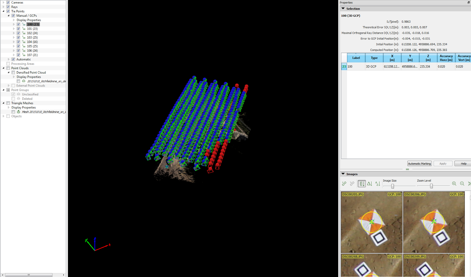
Once the initial processing is complete you will need to reopen the GCP/Manual Tie Point Manager and select rayCloud Editor.  The rayClound Editor will open the GCP display properties on the left hand side and adjustment window on the right side of the screen.(Fig. 8).

(Fig. 8) GCPs display properties (Left) and adjustment window (Right) in Pix4D.

Selecting one of the GCP points from the Display Properties from the left hand menu will open images which contain the GCP marker flag in the right hand Properties menu (Fig. 9).  The blue circle with the blue dot in the middle is where Pix4D believe the center of the GCP point is.  To correct the location you need to select the center of the marker flag.  After selecting the center of the flag in two image select Apply to correct the location based on your corrected locations.  This initial correction will help bring the marker flag into view in all the images (Fig. 10).  The more images your apply correction to the closer the blue circle and dot will become to lining up with the center of the marker flag.  Proceed to select the center of the flag for all the images which contain the marker flag.  Do not selected any point in the images which do not contain the marker flag.  Complete the same process for all of the GCPs from the Display properties menu which will display the number of imags you have corrected after the GCP number in brackets (Fig. 11)

(Fig. 9) GCP marker flags displayed in the Properties window of the rayCloud editor.  The blue circle with the blue dot in the middle is the believed center of the GCP point.  I manually selected the location marked with the  green X and the yellow circle w/plus symbol.

(Fig 10) GCP marker flags after applying the first corrections to bring the other marker flags in to view of the remaining images.

(Fig. 11) Display Properties menu with the corrected image numbers in brackets after the GCP number.

After correcting all of the GCP point locations you can finish the processing by selecting 2. Point Cloud and Mesh, and 3. DSM, Orthomosaic and Index boxes from the Local Processing menu (Fig. 12).

(Fig. 13) Select 2. Point Cloud and Mesh and 3. DSM, Orthomosaic and Index before starting the processing of the images. 

Results

The error for between the two mosaic images is minor when observed in full view.  Had the error been more drastic I could have created a map with both mosaics displaying the variance between the two.  However, when I brought both of the images into ArcMap you could not tell the difference at the extent need to display the entire mine area.  Analyzing where the road connects to the mosaic from the basemap is one of the most noticeable (though very minor) errors with the mosaic (Map 2).

(Map 1) Display of the orthomosaic created with GCPs data.

(Map 2) Display of orthomosaic image created with Geosnap data.

To display the mosaic from a different point of view I created a 3 dimensional (3D) image in ArcScene.

(Map 3) 2D display of a 3D image created in ArcScene of the Litchfield Mine.

Discussion

I first compared the Quality Report of the two projects I ran in Pix4D to see if I could identify the differences.  The majority of the values were the same except when I compared the Geolocation Details.  The report for the project utilizing GeoSnap displays an RMS error of .36-.44 for the various axis (Fig. 12). The report for the project using GCPs showed the RMS error was between 1.01-1.97 for the various axis (Fig. 13).

(Fig. 12) Absolute Geolocation Variance chart from Pix4D Quality Report of the mosaic created without GCP points.

(Fig. 13) Absolute Geolocation Variance chart from Pix4D Quality Report of the mosaic created with GCP points.

Does this mean the GeoSnap is more accurate than using GCPs?

Based on the RMS error one would believe the Geosnap is providing more accurate results.  To make a comparison I exported the GCP coordinates to a feature class in ESRI Arc Map.  Next, I brought in both of the created mosaics for comparison.

(Fig. 14) GCP location (green triangle) and actual GCP location (orange and white triangle) from Geosnap mosaic.

(Fig. 15) GCP location (green triangle) and actual GCP location (orange and white triangle) from GCP mosaic.

After comparing both the mosaics it was easy to see the mosaic created with the GCPs was more accurate than the mosaic created with Geosnap.  I utilized the Georeferance tool in ArcMap to compare the RMS error between the two created mosaics.  The results from ArcMap shows the RMS error of the GCP image is lower than the Geosnap image.

(Fig. 16) RMS Error from the Geosnap mosaic in ArcMap.

(Fig. 17) RMS Error from the GCP mosaic in ArcMap.

Pix4D believes the Geosnap image is more accurate based on the information provided. However, GPS on the camera does not have the accuracy of the GPS unit which collected the GCP locations. The GPS location was collected with a Topcon Hiper and Tesla unit in the same method as I collected point in my topographical survey in my Geospatial Field Methods class.  The Topcon has an accuracy of about 3-5 mm depending on the axis.  The Geosnap Pro model has an accuracy of approximately 1.5 m.

I feel the Geosnap still has applications in the field.  There are many instances where it may not be feasible to layout and collect the information required to produce GCPs coordinates.  In very rugged terrain I believe the Geosnap would really shine through and obtain a high enough level of accuracy for the task at hand.

The above discussion displays why the use of GCPs are more accurate and required when performing flights where highly accurate data is necessary.  In the following labs we will be exploring additional uses with in Pix4D and utilizing the high level of accuracy which GCPs provide.

Processing Pix4D Imagery

Introduction

The purpose of the lab is to introduce me to the software package Pix4D Pro.  Pix4D software has the ability to generate orthomosaic and georeferenced 2D and 3D maps and models from images collected by various methods including UAS platforms.

During this lab I will be creating orthomosaic maps from data captured with two different sensors. The first data I will be processing was collected with a Canon SX260 digital camera.  The second set of data I will be processing was collected with a GEMs sensor.  For more information on the GEMs sensor see my previous blog post.  In the following sections of my blog post I will discuss some of the specifics of Pix4D as answers to questions asked by my professor in the lab assignment.  The following section will give you (the reader) a good understanding of the steps required to process data in Pix4D.

Get familiar with the product (questions in italics)

Look at Step 1 in the software manual (before starting a project). What is the overlap needed for Pix4D to process imagery?

Step 1 in the software manual highlights the proper planning to achieve the highest quality results. Collecting all of the data properly in the field will allow for a streamline process and produce quality mosaic images.  Step 1 in the manual highlights the necessary minimum requirements your data must meet to create mosaic images.

The recommended overlap for most situations is 75% frontal overlap and a minimum of 60% sidelap (Fig. 1).

(Fig. 1) Ideal Images Acquisition Plan for General Cases.

What is the overlap needed if the user is flying over sand/snow, or uniform fields?

Due to snow and sand having large uniform areas it is recommended to have a higher overlap than general landscapes.  The recommendations from the manual is a minimum of 85% frontal overlap and a minimum of 70% sidelap.

What is Rapid Check?

Rapid Check is a feature in Pix4D which allows you to check and see if the parameters set in the flight plan was adequate enough to produce a mosaic image.  Rapid Check reduces the resolution of the captured images to 1 megapixel (MP) to allow for faster processing.  This reduction in resolution leads to lower positional accuracy and can lead to incomplete results.  The manual states, "If Rapid Check succeeds then it is safe to assume that the results of Full Processing will be of high quality." Then the manual states if the Rapid Check fails to run that adjustments to the overlap may be needed. Another option would be to fly the mission again to combine both sets of images to try and achieve success of the Rapid Check.  The manual also states it is possible to run Full Processing on images which fail the Rapid Check but the results may be of a lower quality and could contain erroneous results.

Can Pix4D process multiple flights? What does the pilot need to maintain if so?

Pix4D can process images collected from multiple flights.  There are three parameters you should follow when collecting data with multiple flights.

1. Make sure each flight plan captures the images with enough overlap for the situation.
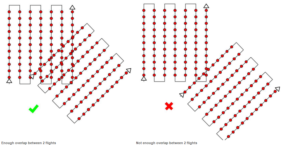
2. Make sure there is enough overlap between the two images for proper correlation (Fig. 2)
3. Make sure the flights are flown in the same conditions like sun angle, weather, and no new features on the surface.

(Fig. 2) Proper and improper overlap between 2 flights display. (Pix4D Manual)

Can Pix4D process oblique images? What type of data do you need if so?

Yes Pix4D can process oblique images.  The example given in the manual is based around constructing a 3 dimensional image of a building.  The instructions state the first flight around the building should be at a 45 degree angle (Fig. 3).  The following flights should increase in height and decrease  the camera angle.  The recommendation is to decrease the angle by 5-10 degrees  per flight to ensure the images have enough overlap to generate the mosaic image.  However, do to variation in spatial resolution you do not want to increase the height more than two times between flights.  Processing oblique images results in a very good 3 dimensional image but does not produce a orthomosaic image.

(Fig. 3) Proper collection of oblique imagery. (Though they don't follow their own instructions) (Pix4D Manual)

Are GCPs necessary for Pix4D? When are they highly recommended?

Ground Control Points (GCPs) are not necessary when processing images in Pix4D.  The use of GCPs improves the global accuracy of the project.  GCPs are highly recommend when processing images which do not have geolocation information.  While you can still process the images without the GCPs your final mosaic output will not have a scale, orientation, or absolute position information.  Without this information you will be unable to complete measurements, perform overlays, or compare previous results.

What is the quality report?

The quality report is like a report card for the images you processed.  The report contains almost every bit of information about the image processing results you could think of.  The first section is a overview of the project and you will see is a Summary, Quality Check, and a Preview (Fig. 4).  The Summary has basic information about the processing such as the name of the project, date and length of time to process, and area dimensions of the processed image.  The Quality Check displays specific information about the calibration results between images.  The Preview displays and 2 dimensional image of an Orthomosaic and a Digital Surface Model (DSM) image created from the processed images.

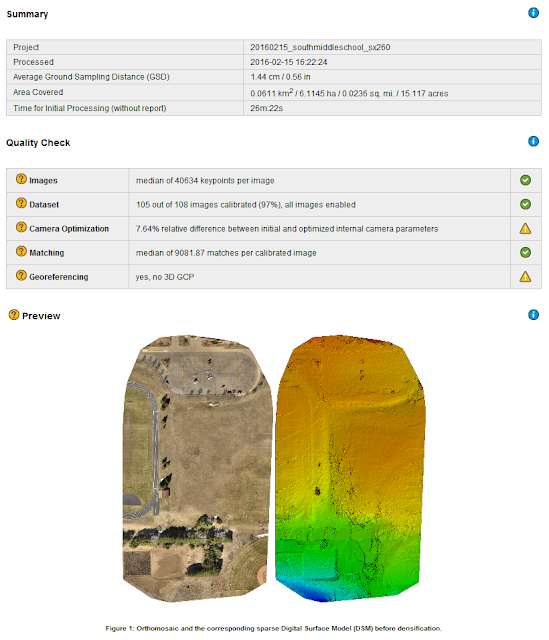
(Fig. 4) First section of the quality report containing the Summary, Quality Check, and Preview.

The second section of the quality report is Calibration Details and contains information about the flight and the images collected during the flight.  The first detail image contained in this section is of the flight path and the locations the images were collected.  The next part image contains a display of the Computed Image/GCPs/Manual Tie Points Positions.  The next section displays the image overlap which the most important details of this section to me as an analyst (Fig. 5).  The higher the overlap the more accurate and the better the mosaic will be.

(Fig. 5) Number of overlapping images reported from the quality report from Pix4D.

The final three sections which include, Bundle Block Adjustment Details, Geolocation Details, Point Cloud Densification details, and DSM, Orthomosaic and Index Details are in depth results of the math which went into configuring the complied image, location accuracy, and processing options with specifications.

Methods

The following steps are completed after the flight has been flown and downloaded your computer. After opening Pix4D select Project and New Project from the menu bar (top left) to open the New Project window (Fig. 6).  From this window you will fill in the name your project and select the location where Pix4D will save the files created during the project process.  Under the Project Type select the New Project and then select Next from the bottom right hand menu bar.

(Fig. 6) New project window in Pix4D.

The next screen you are brought to is the Select Images section of creating a new project (Fig. 7).  From this window you will select the images from the flight which were previously downloaded.  Select Add Images and then locate all of the images you want to be included in the processing then click Next.  After selecting next it will take a brief moment to process the images and proceed to the next screen.

(Fig. 7) Select Images section of creating a new project.

After the image load you will be brought to the Image Properties window (Fig. 8)  The first line in the window will show you the coordinate system which the images are displayed in.  Then next line displays how many of the images are Geolocated.  The third line shows the camera/sensor which was used to capture the image.  Not all sensors are loaded into the Pix4D software.  In this case the GEMs sensor was not loaded in and I had to located the sensor specifications and add them to the image properties using the Edit... button.  I also had to process images collected by a Canon SX260.  When I loaded the images from the SX 260 all of the geolocation information was already attached to the file and loaded automatically.

(Fig. 8) Image properties window of creating a new project without geolocation information.

My example in (Fig. 8) shows none of my images are geolocated.  The images in this window were collected with the GEMs sensor which does not automatically attach the geolocation to the images. This must be done manually by selecting the From File... button which will bring you to the Select Geolocation File (Fig. 9).  From this window you can select the file which contains the geolocation information for the corresponding images.

(Fig. 9) Select geolocation file window.

After adding the geolocation information your the Latitude, Longitude, and Altitude should no longer contain zeros (Fig. 10).  Make sure to check all of your images have been geolocated and filled in.  In the last three projects I have ran in Pix4D I have had one image from each which was not properly located.  When you find which image does not have any location information attached simply uncheck the Enabled check box to exclude it from the process.

(Fig. 10) Image properties window with geolocation information.

With all the information set in the Image Properties window select Next which will bring you to the Processing Options Template (Fig. 11).  From this window you can select what type of project you would like the software to develop.  In my situation I will be creating a 3D Map from the images.

(Fig. 11) Processing options template window.

With 3D Maps selected I clicked next which brought me to the Select Output Coordinate System window (Fig. 12).  I did not change anything in this window and clicked finish to create the project.

(Fig. 12) Select output coordinate system window.

Once the finish button has been selected the flight and location of recorded images will be loaded on a aerial imagery basemap with labels in the processing window (Fig. 13).  From this window to process the image, you have to select the Start button from the Local Processing menu at the bottom of the screen.  The three check boxes which are green in (Fig. 13) will be displayed as red in an unprocessed image.  Once the processing has completed for each section they turn from red to green. Processing time depends on the number of pictures you are utilizing to create the mosaic and the processing power of your computer.  The minimum system requirements recommended by the manufacturer for medium projects (100-500 images @ 14 megapixels) is 8 GB of RAM and 20GB of HDD Free Space.

(Fig. 13) Image processing window with loaded project in Pix4D software.

When completed you should see your processed image with the tie points and camera images displayed along with the Quality Report (Fig. 14).  Examining the Quality Report will tell you the number of images which were calibrated.  For the report displayed in (Fig. 14) I had 105 out of 108 images (97% ) which were calibrated.

(Fig. 14) Post processing display in Pix4D.

Examining the overlap display in the Quality Report (Fig. 5) shows a number of areas where the overlap could have been improved.  The side lap and the frontal lap could have both been increased for better results.  Though the spacing of the images was not quite correct the processing still produced a quality orthomosaic.

Collecting Measurement from the Results

After creating the orthomosaic, one of the tools with the most practical applications is the measurement tools.  The measurement tools allow you to measure straight line distance, area, or volume of a 3 dimensional surface (Fig. 15).

(Fig. 15) Measure tool bar. Straight line distance (Left), Area (Center), Volume (right).

To measure an area after selecting the area measure tool, simply draw a polygon around the feature to measure using as many vertices as necessary (Fig. 16).  Once you have completed the polygon simply right mouse click to end the drawing which will display the measurement in the upper right hand corner of the screen.  The measurement window displays Terrain 3D Length, Projected 2D Length, Enclosed 3D Area, and Projected 2D area.  Below the measurement window is a display of the vertical view of the images with vertices (tie points) in them.

(Fig. 16) Measurement of an island area with in Pix4D.

To measure a straight line distance after selecting the proper tool, simply select the starting point and when you place the cursor on the point you want to measure to use the right mouse button to create the end point.  To display the accuracy of the tool I measure from the start and finish line for the 100m dash at the school track which was in a portion of my image (Fig. 17).  The measurement window displayed a Terrain 3d Length of 100.84 m and a Projected 2D Length of 100.78 m.  When zoomed all the way in I could see my tie point was past the line which explains the variation in the measurement (Fig. 18).

(Fig. 17) Measuring the 100 m dash start to finish line using the straight line distance measuring tool in Pix4D.

(Fig. 18) Overshoot of the tie point for the line measurement.

Measuring volume following the same steps as the previous measurements.  The only difference is when you right mouse click to create the last point it does not automatically update the volume measurement window.  Select Update Measurement button with in the Measurements window. There are various measurement displayed in the window including but not limited to Cut, Fill, and Total Volume.

(Fig. 19)  Volume measurement of a surface in Pix4D.

The last feature in Pix4D I explored was creating a "fly" through animation video of the mosaic image.  Following the help instructions I created way points for the video and the software produced the following video (Fig. 20).  To create a "fly" through animation right click on "Objects" when in the rayCloud menu and select New Video Animation Trajectory.  From this menu you can create your own trajectory or use the flight path records to create the animation.  You have the ability to adjust the speed and duration of the video.  Once finished you can export the animation path you have to Render the video before you export it.

(Fig. 20) Fly through video created in Pix4D.

Results

(Fig. 21) GEMs imagery map mosaic of a pond at South Middle School in Eau Claire, Wisconsin. I exported the measurements made in Pix4D as shapefiles and displayed them on the map. 

(Fig. 22) Canon SX260 map mosaic of a portion of South Middle School in Eau Claire, Wisconsin.

Discussion

Pix4D is very user friendly program to operate.  The methods and tools described above are just basic operations of the program.  One of the most useful functions in Pix4D was the ability to export measurements as shapefiles.  Displaying measurements on maps is a great way to give a sense of distance to the reader.  The help feature and software manual are very useful and easy to understand. When you run into an issue, a simple search leads you to a link with the answers.

The only down side to Pix4D is the amount of processing power and time required to fully process images into a mosaic.  The program will crash conventional computers which have low RAM capacities.

The fly through animation was an interesting feature, but like any video files they take up a long of space.  I created a longer animation video than the one displayed above but could not embed it in Blogger due to size restrictions.

Overall, I am impressed with the Pix4D software.  I look forward to exploring additional tools and uses with in Pix4D throughout the semester.